
✨ ROS 2 C++ Debugging Setup with VS Code
For our developers working in robotics in Berlin with ROS
 Skip to content
 If you’re diving into the exciting world of Robotics, especially in the realm of Autonomous Driving, you’ve likely encountered the ROS 2 localization stack. A crucial, yet often initially perplexing, component within this stack is the covariance matrix. Understanding this mathematical tool – a fundamental concept you’d explore in any comprehensive robotics course Berlin or elsewhere – is key to grasping how your robot perceives its certainty about its position and orientation. Let’s break it down.
At its core, a covariance matrix in ROS 2 localization (and in statistics generally) quantifies the uncertainty and interdependencies of a set of variables. In the context of a robot navigating its environment, these variables typically represent its pose – its 3D position (x, y, z) and its 3D orientation (roll, pitch, yaw).
Think of it like this: your robot’s sensors (IMUs, LiDAR, cameras, GPS) aren’t perfect. They provide estimates, and these estimates come with a degree of doubt. The covariance matrix is a compact way to represent this doubt.
In ROS 2 messages like nav_msgs/msg/Odometry or geometry_msgs/msg/PoseWithCovariance, you’ll find this covariance typically as a 6×6 matrix (a 36-element array). This is because we’re dealing with 6 degrees of freedom (DOF):
Let’s label the rows and columns of our 6×6 covariance matrix corresponding to our pose variables: [x, y, z, roll, pitch, yaw].
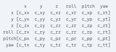
Here's the breakdown:Diagonal Elements (e.g., cxx, cyy, cθθ): These are the variances.
Off-Diagonal Elements (e.g., cxy, cxθ): These are the covariances.
There isn’t a single magic formula. It’s a combination of datasheet analysis, empirical testing, and educated tuning. The goal is to provide a realistic, quantitative measure of your sensor’s noise and uncertainty.
This is the most reliable way to get a solid baseline. The principle is to collect a statistically significant amount of data from a sensor while it’s held stationary and then analyze the spread of the measurements.
Step-by-Step Guide:
Isolate the Sensor: Let your robot remain completely still on a flat surface.
Collect Data: Record the raw sensor output for a few minutes. For an IMU, you might collect several thousand messages. For a GPS, a hundred messages might be sufficient.
Calculate the Variance: Use a simple script (Python with NumPy is perfect for this) to calculate the variance for each variable in the sensor’s message.
Example with Python:
Let’s say you collected 1000 IMU angular velocity Z-axis readings (gyro_z) while the robot was still.
  import numpy as np

# Example: 1000 gyro readings collected while stationary
# In reality, you would load this from a rosbag file.
gyro_z_readings = [...] # Your collected data

# The mean should be close to zero if the sensor is well-calibrated
mean_gyro_z = np.mean(gyro_z_readings)

# The variance is the key!
variance_gyro_z = np.var(gyro_z_readings)

print(f"Calculated Variance for Gyro Z: {variance_gyro_z}")

# This variance value is what you would put in the covariance matrix
# for the (yaw_velocity, yaw_velocity) element.
What about the Off-Diagonals?
For this initial empirical measurement, you can assume the off-diagonal elements are zero. This implies that you’re assuming the noise between variables is uncorrelated (e.g., the noise in the X-acceleration measurement is independent of the noise in the Y-acceleration). This is a very common and reasonable starting point.
Some high-quality sensors, particularly IMUs, provide noise characteristics in their datasheets. Look for terms like:
This method is faster but can be less accurate because datasheet values are from ideal lab conditions, which might not match your robot’s environment (e.g., vibrations from motors).
Start with a reasonable guess. The most important thing for the Kalman filter is the relative ratio of uncertainty between different sensors.
For example, your initial odometry covariance for X might be 0.01, while your GPS covariance for X might be 1.0. This tells the filter to trust the odometry 100 times more than the GPS for high-frequency updates.
“Correct” doesn’t mean perfect; it means the matrix realistically represents the sensor’s behavior. An incorrect covariance matrix will cause the filter to be either overconfident or underconfident.
This is your first and most powerful tool. The robot_localization package publishes the filtered odometry as a nav_msgs/msg/Odometry message, which includes a PoseWithCovariance.
PoseWithCovariance display and subscribe to your filter’s output topic (e.g., /odometry/filtered).What to Look For:
If you have a “ground truth” system (like a motion capture system or RTK GPS), you can perform a more rigorous check.
This is a powerful statistical tool built into robot_localization.
robot_localization documentation provides the expected 95% confidence bounds. If your NIS plot consistently shows values above this bound, it’s a strong statistical indication that the filter is too “surprised.” This means your sensor’s covariance is too small (the filter is overconfident in its predictions).Understanding and correctly utilizing covariance matrices is paramount in robotics for several reasons:
robot_localization) fuse data from these sensors. The covariance matrix of each sensor input tells the filter how much to “trust” that particular piece of information. A sensor reporting high certainty (low covariance) will have a greater influence on the final state estimate.For anyone looking to Learn Robotics Berlin, getting a solid grasp of concepts like covariance is a stepping stone to building more robust and reliable autonomous systems. The precision demanded by applications like Autonomous Driving simply wouldn’t be possible without accurately modeling and managing these uncertainties.

For our developers working in robotics in Berlin with ROS
The world of robotics is undeniably exciting, and getting hands-on