If you’re diving into the exciting world of Robotics, especially in the realm of Autonomous Driving, you’ve likely encountered the ROS 2 localization stack. A crucial, yet often initially perplexing, component within this stack is the covariance matrix. Understanding this mathematical tool – a fundamental concept you’d explore in any comprehensive robotics course Berlin or elsewhere – is key to grasping how your robot perceives its certainty about its position and orientation. Let’s break it down.
What Exactly IS a Covariance Matrix in ROS 2 Localization?
At its core, a covariance matrix in ROS 2 localization (and in statistics generally) quantifies the uncertainty and interdependencies of a set of variables. In the context of a robot navigating its environment, these variables typically represent its pose – its 3D position (x, y, z) and its 3D orientation (roll, pitch, yaw).
Think of it like this: your robot’s sensors (IMUs, LiDAR, cameras, GPS) aren’t perfect. They provide estimates, and these estimates come with a degree of doubt. The covariance matrix is a compact way to represent this doubt.
In ROS 2 messages like nav_msgs/msg/Odometry or geometry_msgs/msg/PoseWithCovariance, you’ll find this covariance typically as a 6×6 matrix (a 36-element array). This is because we’re dealing with 6 degrees of freedom (DOF):
- Position: x, y, z
- Orientation: roll, pitch, yaw
Dissecting the 6x6 Covariance Matrix: What Do the Numbers Mean?
Let’s label the rows and columns of our 6×6 covariance matrix corresponding to our pose variables: [x, y, z, roll, pitch, yaw].
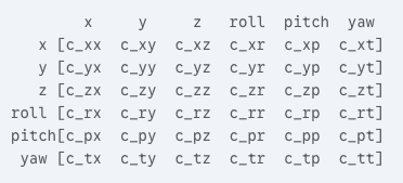
Here's the breakdown:Diagonal Elements (e.g., cxx, cyy, cθθ): These are the variances.
- cxx represents the variance in the robot’s x-position. A smaller value means the robot is more certain about its x-coordinate. A larger value indicates more uncertainty.
- Similarly, cyy is the variance in y, czz in z.
- crr (often denoted as croll,roll), cpp (cpitch,pitch), and ctt (cyaw,yaw) represent the variances in roll, pitch, and yaw orientations, respectively. Again, smaller means more certain.
- Key takeaway: Large diagonal values = high uncertainty in that specific variable. Small diagonal values = low uncertainty.
Off-Diagonal Elements (e.g., cxy, cxθ): These are the covariances.
- They describe the relationship between two different variables.
- A positive covariance (cxy>0) means that if the estimate of x is higher than the true value, the estimate of y is also likely to be higher (and vice-versa). They tend to err in the same direction.
- A negative covariance (cxy<0) means that if the estimate of x is higher, the estimate of y is likely to be lower. They tend to err in opposite directions.
- A covariance close to zero (cxy≈0) suggests that the uncertainties in x and y are largely independent. An error in x doesn’t tell you much about a potential error in y.
- For example, cx,yaw would describe the relationship between the uncertainty in the robot’s x-position and its yaw orientation. This can be significant; imagine a robot moving down a corridor – an error in its yaw (orientation) will likely lead to an increasing error in its perpendicular position (e.g., y-position if x is forward).
Why Does This Matter for Robotics and Autonomous Driving?
Understanding and correctly utilizing covariance matrices is paramount in robotics for several reasons:
- Sensor Fusion: Robots often use multiple sensors. Kalman filters (like those in
robot_localization) fuse data from these sensors. The covariance matrix of each sensor input tells the filter how much to “trust” that particular piece of information. A sensor reporting high certainty (low covariance) will have a greater influence on the final state estimate. - Path Planning & Navigation: A motion planner needs to know how certain the robot is about its pose. If the uncertainty is too high, the robot might need to perform actions to re-localize or move more cautiously. For Autonomous Driving, this is critical for safety – an overconfident but incorrect localization can lead to disastrous decisions.
- Error Propagation: As the robot moves, uncertainties accumulate. Covariance matrices help model how these uncertainties grow and interact over time.
- Debugging and Tuning: If your robot’s localization performance is poor, examining the covariance matrices can provide clues. Are certain sensors consistently reporting very high uncertainty? Are there unexpected correlations between variables?
For anyone looking to Learn Robotics Berlin, getting a solid grasp of concepts like covariance is a stepping stone to building more robust and reliable autonomous systems. The precision demanded by applications like Autonomous Driving simply wouldn’t be possible without accurately modeling and managing these uncertainties.